Math and Measurement

Finding Connections in Data
It is the aim of physics to understand how the physical universe works. A scientist explores the universe through observation and experiment. By carefully examining the data collected in an experiment it is possible to understand how different aspects of the physical universe interact with one another.
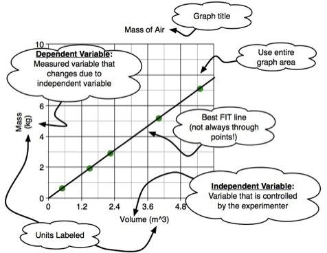
Constructing a graph from experimental data is a powerful tool which is useful in determining the relationship between the variables of an experiment. There are certain expectations when experimental data is presented on a graph:
- A graph should have a title explaining the data it presents.
- The axii of the graph should be clearly labeled with units explicitly noted.
- The dependent variable is the quantity that is directly manipulated by the investigator doing the experiment. Data for the dependent variable should be plotted on the horizontal axis of a graph.
- The independent variable is the quantity that responds to changes in the dependent variable. Data for the independent variable should be plotted on the vertical axis of a graph
- A best-fit line drawn by inspection would have an equal number of data points above and below the line.
- The resulting equation for any mathematical fit to the data should be noted on the graph
The data from an experiment is often organized into a table before it is plotted. Consider an experiment to determine the density of air by measuring how the mass of a sample changes when the volume of the sample is increased.
| Table: Collected Volume and Mass Data |
|
| Volume of Air (m3) | Mass of Air (kg) |
| 1.45 | 1.98 |
| 2.30 | 2.92 |
| 4.02 | 5.18 |
| 5.24 | 7.11 |
When plotted, the data produces the graph shown in Figure 1.

Figure 1: The parts of a properly constructed graph.
Common Relationships in Data
Not every experiment leads to a clear picture of the relationship among the variables observed in the investigation. However, there are some common behaviors found throughout the physical world. It is often possible to spot the behavior shared by variables by examining the data plotted on a graph.
Linear
The relationship between variables is said to be linear if data can be best fitted by an equation of the form
y = mx + b
Where x, y are the independent and dependent variables, b is where a line would cross the vertical axis (x = 0) and m represents the slope of the line

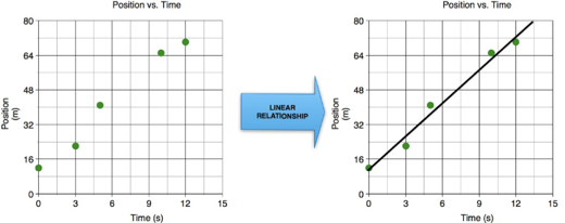
A common example in physics of a linear relationship is how the position (x) of an object changes in time (∆t) when moving at a constant velocity (v)
x = x0 + v ∆t
A graph of position and time data is shown in Figure 2.

Figure 2: Variables with a linear relationship.
Quadratic Relationship
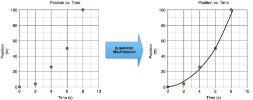
If the velocity of an object is not constant, but is accelerated (a) the relationship between a change in position (∆x) with respect to changes in time (∆t) is quadratic, with the following relationship
∆x = 0.5 a (∆t)2
A graph of position and time data is shown in Figure 3.

Figure 3: Variables with a quadratic relationship.
Inverse Relationship
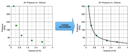
An inverse relationship is when two variables always multiply to the same constant value (often written as 'k') . If the temperature of an ideal gas does not change, the pressure (P) and volume (V) share an inverse relationship (known as Boyle's Law)
PV = k
The equation can be rearranged to read
P = k / V
A graph of position and time data is shown in Figure 4.

Figure 4: Variables with an inverse relationship.